SIGNA MR355 / SIGNA MR360
Service Manual
5856356-3EN Revision 5.0
Basic Service Documentation. Copyright General Electric Company.
Object ID: 00000018WIA30D37E20GYZ
Topic ID: id_13107100 Version: 3.0
Date: Aug 29, 2019 1:36:27 AM

Grafidy Manual Mode Procedure

Prerequisites

Table 1. Personnel requirements
Required persons	Preliminary requirements	Procedure	Finalization
1	-	-	-

Table 2. Safety

Table 3. Required conditions
Condition	Reference	Effectivity
The Automatic Mode Should be Used for most proposes. Only use manual mode if required for touch up.	-	-
System has bee configured and configuration tested in order to run Grafidy 3	-	-

Manual Mode

About this task

If for some reason the Auto Mode procedure does not bring one or more of the numeric output final values of your system completely into specification, you may continue adjusting the out-of-specification values using Manual Mode.

Procedure

After the Auto Mode scanning is complete, choose the Manual Mode Tab. See Figure 1.

Figure 1. Manual Mode Tab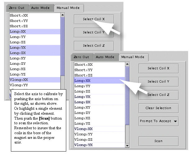
Set the coil in the magnet on the scan axis desired, then highlight the scan components that you would like to perform (i.e. click on “Long XX”, or alternatively, click “select coil X” for xx, yx, zx of long and very long) and press “scan”. See Figure 1.

The naming convention for a component is: the first letter refers to gradient axis, the second letter refers to coil axis (for example, yx means gradient is on the y axis, but the coils should be placed onthe x axis). Make sure the coil axis in the magnet and the selection are consistent.
After the scan is complete, a plot window will pop up that is similar to the one in Figure 2. Notice that there are two buttons that read Accept and Cancelin the lower right corner.

Figure 2. Results Window with Accept/Cancel Buttons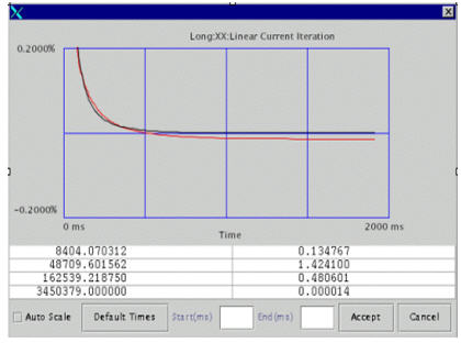
Choosing Accept will overwrite the previously-stored values in the calibration files (grafidyx.cal, grafidyy.cal and grafidyz.cal). Either Accept and scan again, or Cancel (to leave the values in the cal file/hardware from last accepted iteration) and stop.
If a “good fit” is shown (that is, residual eddy currents are getting smaller), click the Accept button to accept the output calibration parameters, and do another scan. The next measurement is likely to get rid of much of the residual eddy current present in this measure and improve output/result numbers.
If a “bad fit” bad fit is shown (that is, residual eddy current are increasing), click the Cancel button because a bad fit is not likely to improve output numbers for the next measurement.
The last iteration for any component should be check only and therefore should not accept the fitting cal parameters.

Examining a Fit

Procedure

Refer to Figure 3. If the two lines plotted appear to be similar in shape, the fit is probably good. To get a closer look at any one plot, you can choose the “Auto-Scale” function (the auto-scaled fit may appear to worsen as the display scale changes).

To focus on the front of the plot only, choose an End point (e.g., 100 ms). The default is 2000 ms.

Figure 3. Examining a Fit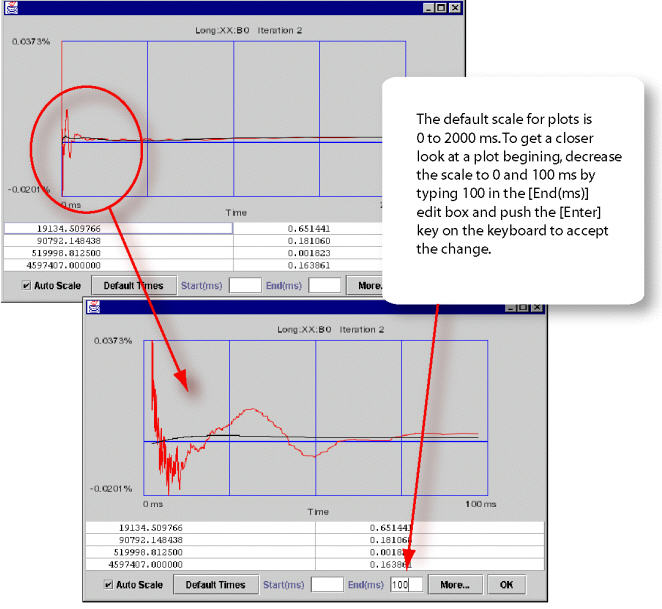

Figure 3 has the same plots except the first one uses default time scale (0 to 2000 ms) and the second one uses time scale of (0 to 100 ms) therefore enlarged the portion of 100 ms.

It is interesting to note that the measured curve (red) and fitted curve (black) in the Figure 3 example have very little in common (especially at the first 100 ms, where the fitted curve is cutting through the measured curve). So, it is very unlikely that any further iteration will improve eddy current compensation and get rid of the “oscillatory” behavior of the start portion of the plot. In this case, system limits have been reached. If the curve of the black line more closely matched that of the red, then another iteration would most likely improve eddy current compensation.
To set the vertical scale in “non-auto scale mode” to a set of values, in addition to the default value 0.2, by right clicking the “drawing area” of the pop-up and then selecting the scale you want. This is useful when you want to do a side-by-side comparison on the same scale other than default. See Figure 4.

Figure 4. Setting Auto-Scale Mode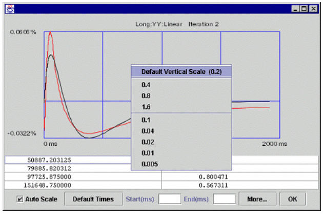

Accept Policies

Procedure

There are 3 accept policies in manual mode: Prompt to Accept, the default, Always Accept or Never Accept. See Figure 5
Figure 5. PROMPT TO ACCEPT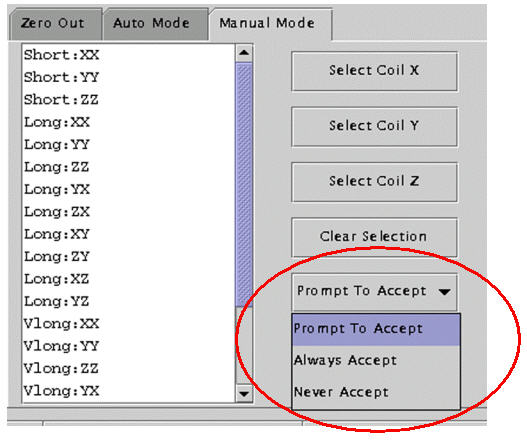
- > Prompt to Accept > will show you what a fit looks like. Based on how good the fit looks, you can decided whether to accept or not.
- > Always Accept > will always accept the fitted cal values. New values are accepted automatically without further intervention.
- > Never Accept > will never accept the fitted cal values. This is useful when you're doing a “check only.”
Continue to Conditions Column

Conditions Column

Procedure

If a cell in the column “Conditions” is selected (long xx linear in this example), and then you click the Show button, you'll see a pop-up like the one shown in Figure 6 (along with the first iteration’s popup). The pop-up lists:
Figure 6. CONDITIONS CELL [SHOW] EXAMPLE POPUP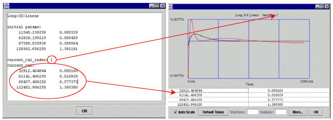
- Initial cal values (initial parameters) of the component (long xx linear in this example) (the cal values of the component when Grafidy 3 was invoked). See Selecting Previous Interations for more information.
- The current cal index = 1, which means that currently the cal values in the cal file (gafidyx.cal) and in the hardware/pre-emphasis were generated by iteration 1, and
- The current cal values are also listed.
When an iteration (iteration 1 in this example) is finished for a component, and if the cal values are “accepted” into the cal file/hardware, the user will see current_cal_index equals to the last iteration number, and current_cal will be the same as contained in the popup of the last iteration (iteration 1 in this example) of the component.
Special cases:
- Current cal index = 0: initial cal values is in the cal file/hardware.
- Current cal index = -1: cal values are set to zero for the component.
- Current cal index = -2: cal values are set to default (short time constant only).
Return to the main menu

Finalization

No finalization steps.