- Discovery MR750 3.0T System Service Methods
- 5690009-2EN Revision 4
- 00000018WIA30BF3E20GYZ
- id_131065873.3
- Aug 26, 2020 1:22:03 PM
RFA loopback test
Prerequisites
| Required persons | Preliminary requirements | Procedure | Finalization |
|---|---|---|---|
| 1 | - | 20 to 60 minutes | 10 minutes |
| Item | Quantity | Effectivity | Part number | Manufacturer |
|---|---|---|---|---|
| RF cables kit | 1 | - | - | - |
| Oscilloscope | 1 | - | - | - |
| Standard tool kit | 1 | - | - | - |
| RF power measurement kit | 1 | - |
One of the following: 5307511-2, 5307511-3, or 5434817 | - |
| Universal SST kit (1.5T and 3.0T) | 1 | - |
5110731-4 | - |
| Head coil | 1 | - |
5180918 | - |
| 200–watt 30 dB attenuator (used as the 1.5T dummy load, secondary, from 1.5T tool kit, 46-317724G1 or 46-317724G2) – For use with dual drive systems ONLY | 1 | - |
46-317724P14 | - |
| 6 feet of N-male to N-male RG214 cable (from 1.5T tool kit, 46-317724G1 or 46-317724G2) | 1 | - |
46-317724P9 | - |
| 70 dB, with 10 dB step, attenuator (from 3.0T grafidy kit, 2386042) | 1 | - |
46-255838P2 | - |
| BNC M-F feedthrough with DC blocking cap (from DVMR service cables kit, 5306523) | 1 | - |
5160682 | - |
| Body sphere (27 cm) | 1 | - |
2359877 | - |
| Body loader | 1 | - |
2360037 | - |
| Head sphere (17 cm) | 1 | - |
2360025 | - |
| Head loader | 1 | - |
2360031 | - |
| Head loader positioner | 1 | - |
5110241 | - |
| Loop Velcro squares (for attaching the RF sense loops; from universal SST kit, 5110731) | as needed | - |
46-307152P1 | - |
| ||||||||
About this task
The RFA (radio frequency analysis) tool is designed to quantitatively measure the performance of the transmit chain by allowing loopback tests from several different points along the chain. At most points, the inter-pulse RF stability and inter-pulse RF fidelity (magnitude and phase linearity) can be measured.
For information about the theory behind the tests, see RF Loopback Test Theory.
Set up test
Procedure
- On the driver module in the PEN cabinet, set switch 2 (SW2) to TR DISABLE.
Figure 1. Setting TR disable 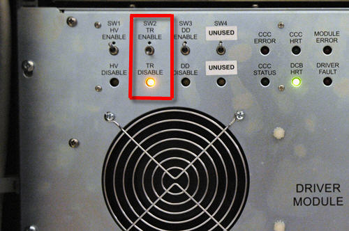
- On the exciter/ref clock module located in the PEN cabinet,
set the RF Enb switch down (Disable).
Figure 2. Exciter/Ref Clock Module 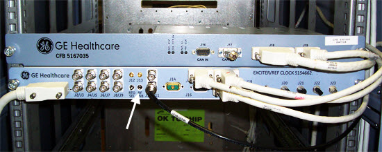
Perform test
Running RFA in exciter, bodydummy, or headdummy mode
Procedure
- In the service browser, select Image Quality > RFA
Tool. The RF Analysis Tool appears.
Figure 3. RF analysis tool (single drive RF amplifier) 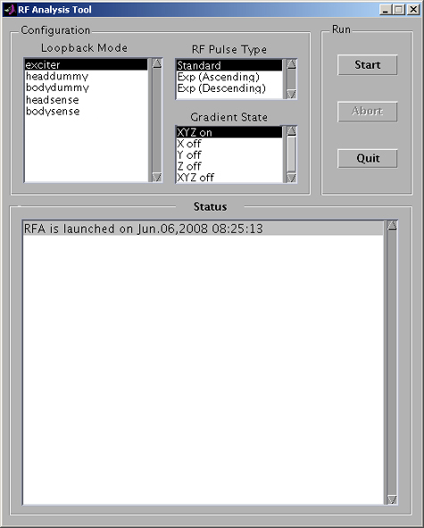
Figure 4. RF analysis tool (dual drive RF amplifier) 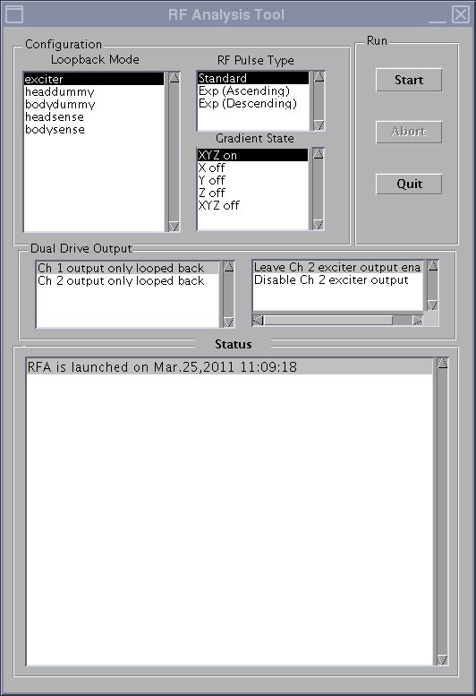
- After about 60 seconds, a Set loopback signal level message box appears. When this message appears, click the Patient
icon.
Figure 5. Patient icon 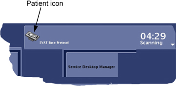
- When done, select the Toolbelt icon to return to the service
window. Start a scan by clicking Proceed & auto-scan on the Set loopback signal level message box.
Figure 6. Message box 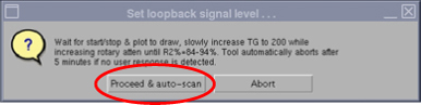
Running RFA in headsense or bodysense modes
Procedure
- After about 60 seconds, a Set loopback signal level message box appears. When this message appears, click the Patient
icon.
Figure 7. Patient Icon
RFA plot results
Inter-pulse stability plots
About this task
The following sample plot results are Inter-pulse Stability (created in Standard Test mode only)
Procedure
- Note: (For systems with dual drive RF amplifiers) There are no specifications for RFA at this time. However, if troubleshooting body transmit issues, both channel 1 and channel 2 should have similar results. There should also be similar results when running RFA on channel 1, with channel 2 active or not active.PkMag
The resulting plot should look similar in magnitude and shape to that shown in Figure 8, Figure 9, and Figure 10.
The title of this plot indicates that it is an RFA tool result (from raw data file /usr/g/mrraw/P04608.7.RFA.exciter) from an exciter loopback test performed with R1=11, R2=12, TG=200, showing RF pulse PkMag results ordered in time.
PkMag means that for each RF pulse we are plotting a point representative of its peak time domain magnitude measured during its play out. This RFA acquisition collected 15 slices worth of RF2 pulses. That is, 15 echo trains per TR period, each train 8 echoes in length, for 32 TR periods or shots (that is, ymatrixSize/teal = 256/8 = 32 shots) for a total of 15x8x32=3840 RF pulses (total plot points).
All data from the first echo train slot in each TR period is shown in a “pure” blue plot with all 256 points acquired for that slot (one per RF pulse) shown in time order from left to right (that is, indices 1 to 256=ymatrixSize on the horizontal axis). All data from echo train slots 2 through 14 in each TR period is shown in separate overlaid plots that gradually change in color from blue to purple to red. All data from the last (15th) echo train slot in each TR period is shown in a “pure” red plot overlaid on all previous plots.
The ideal result showing no problems would appear as a single red horizontal line at a vertical axis value of 100, meaning that every RF2 pulse played for every slice had exactly the same peak magnitude and all these values scaled to 100.0 when the entire data set was normalized to “percent of peak value”. This display format allows visual assessment and separation of instabilities that are tied to echo train, to shot (TR period), to slice time slot, or to the entire scan’s acquisition. Be aware that the plots are auto-scaled.
Figure 8. PkMag, or peak magnitude (exciter) 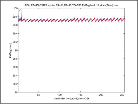
Figure 9. PkMag (body dummy) 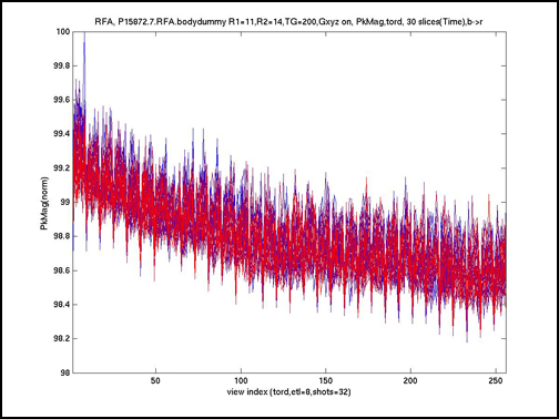
Figure 10. PkMag (head dummy) 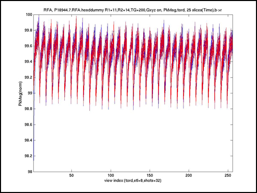
-
Integ
The resulting plot should look similar in magnitude and shape to that shown in Figure 11, Figure 12, and Figure 13.
This is analogous to the earlier PkMag plot description; however, this plot represents the RF pulse INTEGRAL (or area) for each RF pulse acquired.
Figure 11. Integ, or integral (exciter) 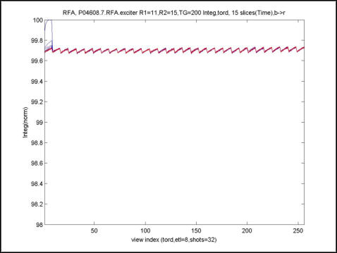
Figure 12. Integ (bodydummy) 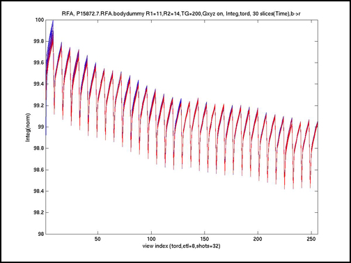
Figure 13. Integ (headdummy) 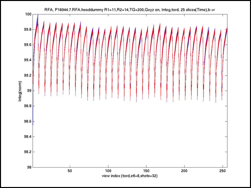
-
0-order Phase
The resulting plot should look similar in magnitude and shape to that shown in Figure 14, Figure 15, and Figure 16.
This is analogous to the earlier PkMag plot description; however, this plot represents the RF pulse 0-order phase (AVERAGE PHASE) in degrees for each RF pulse acquired.
Figure 14. 0-order phase (exciter) 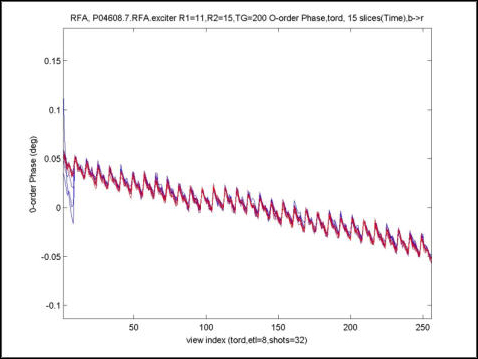
Figure 15. 0-order Phase (bodydummy) 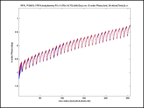
Figure 16. 0-order phase (headdummy) 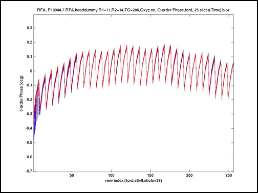
-
1-order Phase
The resulting plot should look similar in magnitude and shape to that shown in Figure 17, Figure 18, and Figure 19.
This is analogous to the earlier PkMag plot description; however, this plot represents the RF pulse 1-order phase (LINEAR PHASE) in degrees/point for each RF pulse acquired.
Figure 17. 1-order pulse (exciter) 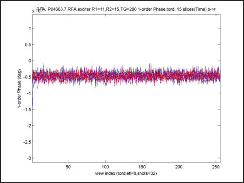
Figure 18. 1-order pulse (bodydummy) 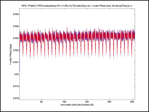
Figure 19. 1-order pulse (headdummy) 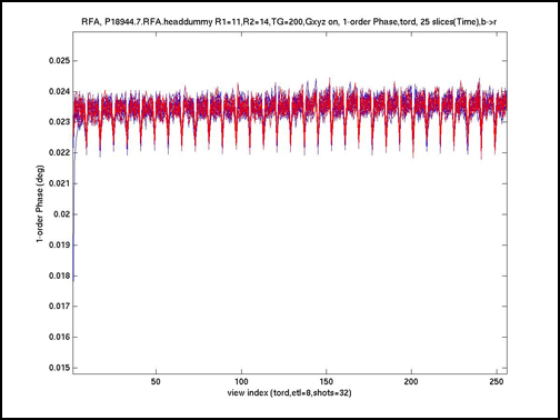
Intra-pulse fidelity plots
About this task
The following sample plot results are Intra-pulse Fidelity (created in Exp(onential) Test mode).
Procedure
-
Magfit
The resulting plot should look similar in magnitude and shape to that shown in Figure 20.
Plot title: none; mag & fit vs sample index; Ideal: Perfect exponential of blue points with overlaid red exponential curve fit.
Plot title: none; mag err(%) vs sample index; Ideal: Flat horizontal blue line of processed points with overlaid flat red curve fit, both at mag err(%) = 0.0 %.
Plot title: none; mag err(dB) vs sample index; Ideal: Flat horizontal blue line of processed points with overlaid flat red curve fit, both at mag err(dB) = 0.0 dB.
Figure 20. Magfit, or intra-pulse (All) 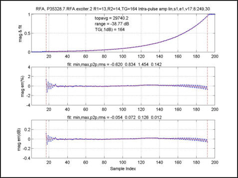
-
Magdif
The resulting plot should look similar in magnitude and shape to that shown in Figure 21.
Plot title: Mag linearity err(%) ; mag err(%) vs dB; Ideal: Flat horizontal blue line of processed points with overlaid flat red curve fit, both at mag err(%) = 0.0 deg.
Plot title: Mag linearity err(dB); mag err(db) vs dB; Ideal: Flat horizontal blue line of processed points with overlaid flat red curve fit, both at mag err(dB) = 0.0 dB.
Plot title: Mag linearity err DIF(dB/dB); mag err DIF(dB/dB) vs dB; Ideal: Flat horizontal blue line of processed points with at mag err(dB) = 0.0 dB.
Figure 21. Magdif (All) 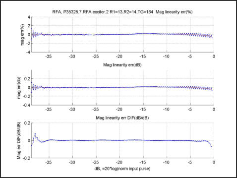
-
Phafit
The resulting plot should look similar in magnitude and shape to that shown in Figure 22.
Plot title: none; Phase(deg) vs sample index;Ideal: One horizontal red line at any phase(deg) value.
Plot title: none; Phase(deg,blue) vs sample index; Ideal: One horizontal red line at same phase(deg) value as previous ideal plot.
Plot title: none; Phase err(deg,blue) & fit(red) vs sample index; Ideal: One horizontal red line at 0.0.
Figure 22. Phafit (All) 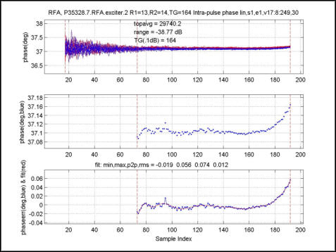
-
Phadif
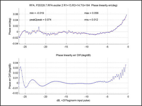
The resulting plot should look similar in magnitude and shape to that shown in Figure 23.
Plot title: Phase linearity err(deg); Phase err(deg) vs dB; Ideal: One horizontal red line at 0.0
Plot title: Phase linearity err DIF(deg/dB); Phase err DIF(deg/dB) vs d; Ideal: One horizontal red line at 0.0
Figure 23. Phadif (All)