Grafidy 3 Procedure
Prerequisites
Grafidy 3 will require 3 hours for a BRM system and 6 hours to complete both WHOLE and ZOOM on a TwinSpeed System.
IMPORTANT! Perform an L-Coil Calibration before starting the Grafidy 3 Procedure: From the Calibration menu, select L-Coil Calibration. Click the selection to start the tool. The calibration runs automatically.
1 Start-Up and Zeroing Values
Procedure
- This procedure documents using the Browser, but this tool is still accessible through the tool menu. Go to the Service Desktop and start the Service Brower, if it is not already started, by clicking Service Browser button on the left tool bar.
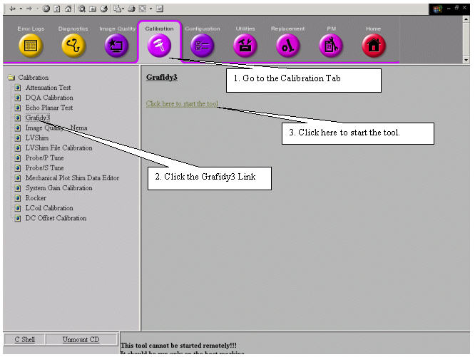
- On the Service Browser start the Grafidy3 calibration. See Figure 1 for instructions.
Figure 1. Starting the Grafidy 3 Tool
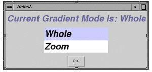
- The Grafidy3 window will first open with a selection box to
set the gradient mode for Grafidy 3, if it is a twin gradient system
(TRM). Choose between Whole or Zoom modes by clicking the appropriate
selection and clicking the OK button. See Figure 2. For systems with a TRM, both Whole and Zoom have to be calibrated.
To switch mode, exit Grafidy 3, and then restart it and select the
next mode to calibrate.
Figure 2. Selecting Gradient Mode
- Next, select the Zero Out tab. See Figure 3.
Figure 3. Zeroing Old Cal Files
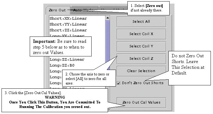
You can select all (components) by clicking the Select All button, or select coil X axis only (xx, yx, zx linear and xx b0 for long and very long), or coil Y axis only, or coil z axis only. You can clear selections, too.
You can also select an individual component (e.g., long xx linear) or components (e.g., long xx linear, and long xx b0) by holding down the Ctrl key on as you click the components on the list.
The selected components are highlighted. The selection itself will not zero out anything. Click theZero Out Cal Values button to actually zero out cal values in cal files (grafidyx/y/z.cal).
The naming convention for a component is this: the first letter refers to the gradient axis, the second letter refers to the coil axis, for example, yx means the gradient is on the y axis, but the coils should be placed on the x axis.
- It is not always required to zero Cal values. It is less time-consuming
and advisable to touch up vales when possible. If you meet any of
the following criteria, click the axis button that needs to be cleared
out, or click the Select All button and then
click the Zero Out Cal Values:
-
If you are working with a new or new system upgrade, zero out the cal values.
-
If the previous eddy current calibration was done using ECMT, zero out the cal values.
-
If the previous eddy current calibration was done prior to Signa software revision 9.0, zero out the cal values
-
If, after attempting to touch up (calibrated eddy current without zeroing out the cal values), values did not converge/specifications not met, zero out the cal values.
-
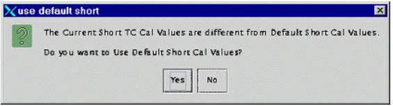
- Use default short time constant cal values rather than calibrating
short TC on a system-by-system basis. When you click either “auto
mode” or “manual mode” (first time per tool invocation),
the tool will check whether the short TC cal values are the same as
the default values. If not, the Grafidy 3 tool will display a message
asking if you want to use Default Shorts Cal Values. Answer Yes. See Figure 4.
Figure 4. Default Short Cal Values Popup
By default, short time constant eddy current are not calibrated. Instead, a set of default calibration values are used. Those values depend on a gradient coil (brm/crm/trm_whole/trm_zoom) and gradient driver (ACGD/ACGD_Lite) combination. Grafidy 3 will check/load proper short TC cal values based on the system configuation.
2 Calibration Scans
Procedure
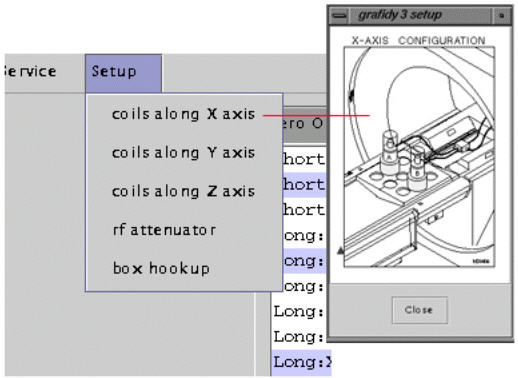
- Position the coils in the magnet bore for the axis to be calibrated.
A diagram of proper coil positioning can be viewed from the menu bar
under Setup by selecting the axis that will
be calibrated. See Figure 5.
Figure 5. Setting Axis to Calibrate
- Click on the Auto Mode tab
- Select the axis that is consistent with the coils set up in the magnet bore and then click the Scan button. The Scan will be grayed out and the Abort button will be activated until the scan is either finished or aborted.
- Only one plane can be calibrated at a time. After the completion
of a plane, the Grafidy coils must be switched to the next plane to
be calibrated and the scan started again. See coil plane configurations.
Each axis will take approximately 60 minutes to complete. See Figure 6.
Figure 6. Auto Mode Setup
- Each component of the axis (e.g.. long:xx, long:yx, long:zx, vlong:xx) will run a maximum number of iterations; by default, 5 iterations for long and 5 for very long . Also by default, short TC is not selected (therefore will not be calibrated). If a target (about half of the spec for long on-axis) is reached before the maximum number of iterations is reached, the system will stop doing iterations for the component.
- As each component finishes an iteration of scan/analysis, the residual eddy current of the measurement will show up in the result area/table. The output of the result will be color-coded. Red text indicates values out of spec. Green indicates values within.
- Review the numeric output values from the auto mode scan. Verify
that the results of final iteration for each component are within
spec. See Figure 7 for help in reading
output values.
Figure 7. Reading Output
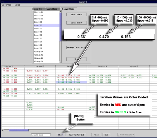
- You can check the eddy current measurement and fitting by clicking
in any cell that has values filled in. Then click the Show button. Refer to Illustration XX for interpreting graphical data.
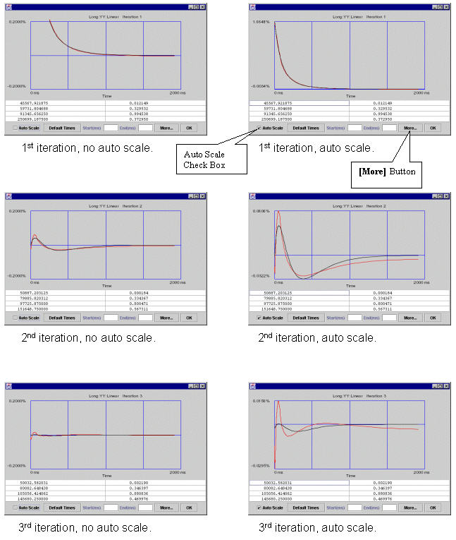
In the left column with auto scale turned off (so they have same vertical scales) from the 1st to the 2nd to the 3rd iteration, the residual eddy current become smaller and smaller.
In the right column from the 1st to the 2nd to the 3rd iteration, viewing the data in Auto-Scale to spread the plot views out (the plot is scaled from minimum values to maximum values, for the 1st iteration the scale is ~1.8, 2nd iteration ~0.06, 3rd iteration ~0.015 in this example). While the residual eddy current becomes smaller when iterations are going on, the quality of the fit between measured curve and fitted curve (goodness of fit) becomes poorer. When those two curves have little in common, which is seen in iteration 3, it is not likely that any further iterations will improve much, and it is time to stop iteration because the system limit has been reached.
Figure 8. Interpreting Grafidy Plots
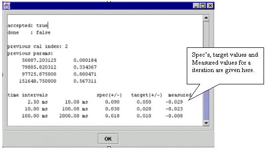
- Click More to show coil positions, spec
values, target values and measured values. See Figure 9 and Figure 10. You will need to
scroll UP to get to the position values.
Figure 9. Coil Position
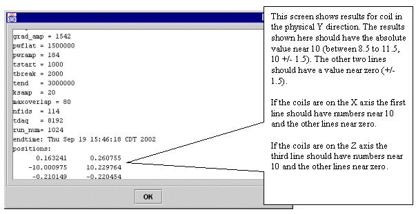
Figure 10. Stem Specs, Target and Measured Values
- If a component is not in spec after the maximum number of iterations, you will need to use manual mode to calibrate that component. See Manual Prescan Mode for help in that procedure.
- Repeat the calibration procedure for all three axes. Always ensure the physical coil axis matches the selected scan axis or errors will result.
- After all three axes are done, re-position the coils and re-scan
long on-axis components other than the last scanned on-axis component.
For example, if the order of the axes scanned is x,y,z, and after
last axis (z) is done, you will need to re-scan long xx and long yy.
Long xx b0 and long yy b0 may be out of spec again (due to cross terms).
If this is the case, do another scan until they are in spec again.
The final step (12) is best suited for manual mode.
3 Finalization
Finalization
No finalization steps.