
- Optima MR450w BASE 1.5T System Service Methods
- 5690012-2EN Revision 3
- 00000018WIA30F1B030GYZ
- id_123741021.7
- Jul 5, 2019 10:03:33 PM
ACR Accreditation Scan Troubleshooting
MR ACR accreditation is offered by the American College of Radiology (ACR). The intent of the program is to ensure a baseline quality standard for all MR diagnostic imaging devices. Accreditation is becoming more important as more and more health care insurance providers are requiring some form of accreditation as a prerequisite to procedure reimbursements. Scanners are assigned accreditation on an individual basis. Sites must submit ACR phantom images using the ACR sagittal localizer, T1, and T2 protocols as well as phantom images using the site’s own routine T1 and T2 scan protocols.
This document provides assistance in performing the ACR phantom scanning with ACR sagittal localizer, T1, and T2 protocols and analysis on GE 1.5T and 3.0T cylindrical scanners, and illustrates the issues that may be encountered. Tips for 1.5T and 3.0T Cylindrical Scanners provides tips on specific issues that might effect this scanning procedure.
Prerequisite: Complete system calibration (clinically ready).
No service key is needed for this procedure.
ACR Phantom Scanning
Most failures in ACR phantom image analysis come from improper phantom positioning and errors in landmarking and/or slice locations. It is critical to properly align the ACR phantom before performing the ACR scans so the slice locations are properly placed on the internal phantom structures.
Taking time to properly position the phantom reduces the time needed to perform these procedures. Setup is an iterative process, with phantom repositioning between each scan, repeated as many times as necessary to center the phantom in all three planes.
During this procedure, several measurements need to be taken and recorded. Use this form to record the ACR Accreditation Scan measurements. 4964620.pdf
ACR Phantom
The ACR phantom must be purchased from the ACR.
Some phantoms have a bubble level viewer that aids the user to correctly position the phantom. It will be located on small shelf that sits about midway under the chin position.
ACR Phantom Positioning: Introduction
This procedure is written to be used with all ACR-compatible head coils.
Ideally, the site should select the head-type coil they use most often for routine clinical head imaging for this ACR phantom scanning. If the ACR phantom does not fit in that coil, try the next most commonly used head-type coil for clinical head imaging, until you find one that fits. This may default to their TR head coil (split-top head coil).
The ACR phantom scanning consists of the following:
-
FGRE 3-Plane 2D localizers (3 images each), with phantom repositioning between each
-
ACR sagittal localizer scan (explicitly prescribed, one sagittal slice)
-
ACR T1 series (graphically prescribed, 11 slices, 11 images)
-
ACR T2 series (same graphic Rx as ACR T1 series, 11 slices, 22 images)
Phantom Setup
If using a curved table, do not use foam service filler panels. The patient cradle should be at its normal clinical imaging height.
-
Place the chosen head-type coil onto the patient cradle, into its normal clinical imaging position, and plug it in. Align, clamp, fasten, etc. the coil using only those method(s) used to place it for routine clinical imaging. Make sure the coil is not off center or rotated from its normal correct position.
-
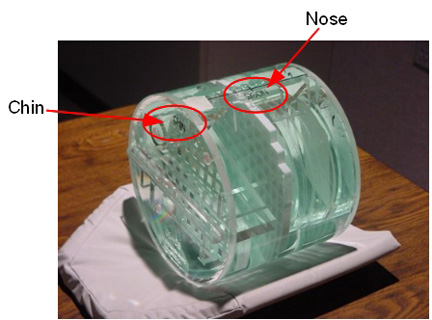
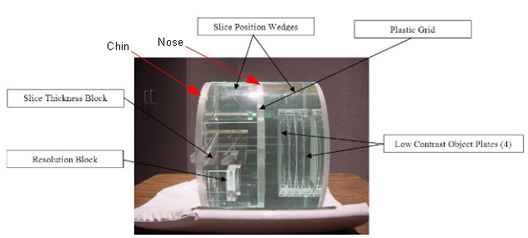
Obtain the ACR large phantom (see Figure 1).
The phantom has both CHIN and NOSE markings that are placed where a patient’s chin and nose would be within the head-type coil for a head first, supine patient orientation. In this procedure, all ACR scanning is done with the head first, supine patient orientation. Therefore, the anterior/posterior (A/P) direction is perpendicular to the patient cradle, along the vertical direction with respect to the floor, along the physical Y gradient. The right/left (R/L) direction is along the physical X gradient direction. The superior/inferior (S/I) direction is along the physical Z gradient direction (in/out of the magnet bore, along magnet B0).
Notice -
You will need something to raise and hold the phantom in a stable position with high spatial precision.
Some sites may have a special positioner intended for the ACR phantom in a particular head-type coil; however, we have often found these positioners to be flawed and/or poorly adjusted. If that positioner does not allow you to accomplish exactly what is described in this procedure, then put it aside.
White printer paper (without any printing or ink/toner on it) is the recommended stable, low compression, high resolution positioning material. You may need more than one stack and/or some folded paper “shims” to accurately position the phantom. Other foam or pads (non-ferromagnetic) may be used as well.
Label and keep what you use so you do not have to re-measure or adjust things much for future ACR phantom scans.
-
Physically center the ACR phantom at the center of the RF head type coil, along all three patient dimensions, before landmarking. This helps avoid axially asymmetric RF “bite marks” in the axial phantom images caused by uneven RF head type coil conductor proximity when the phantom is offset, especially along R/L or A/P.
Line up the ACR phantom’s black S/I center marker with the head type coil’s center along S/I (Z). The amount of positioning adjustability will depend on which head type coil is being used.
Notice Figure 5. Protrusion and Landmark on Head Coil 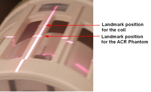
-
Go to the table foot and visually estimate the R/L and A/P centering of the phantom with respect to head type coil center, and reposition the phantom as needed to center it along R/L and A/P. Use a non-ferromagnetic ruler if you think you need it. Also physically align the phantom so it is not rotated about the Z axis (using the phantom’s chin side external bubble level if present) and not rotated about the X or Y axes. The amount of positioning adjustability will depend on which head type coil is being used.
Do the best you can by eye, while monitoring whether one adjustment has compromised another and compensating accordingly. You will readjust the phantom again more precisely later. Iterative 3-plane localizer FGRE scans will be used, with phantom repositioning between each, to ensure that the phantom is centered and aligned.
Landmark/Scan
Use either predefined prescription (Using Predefined Protocols) or manual prescription (Using Manual Protocols).
If the predefined prescriptions are not correct in your system, use the manual settings.
Using Predefined Protocols
-
Landmark precisely on the ACR phantom’s black S/I center line and select Advance To Scan.
-
Select New Patient and use the following parameters:
-
Name: ACR-head type coil name (example: ACR-8HRBrain)
-
Patient ID: ACR-head type coil name (example: ACR-8HRBrain)
-
Weight: 50 lbs.
-
-
Select Show All Protocols.
-
For Protocol Library, click GE
-
On the Other tab, open either the Phantom: Rcv Head Coil folder or Phantom: T/R Head Coil folder, then select a FGRE_3 Plane Localizer series, and then click the right arrow button.
-
Under Multi Protocol Basket, select a FGRE_3 Plane Localizer series, and then select Accept.
-
Click Start Exam.
-
If choices appear, select dB/dt=First level, SAR=First level, and then select Accept.
-
Save the series, and scan.
Using Manual Protocols
-
Landmark precisely on the ACR phantom’s black S/I center line and select Advance To Scan.
Note:If you are on a TWIN gradient system, use either WHOLE or ZOOM gradient mode exclusively. Do not switch modes between any series.
-
Select New Patient and use the following parameters:
-
Name: ACR-head type coil name (example: ACR-8HRBrain)
-
Patient ID: ACR-head type coil name (example: ACR-8HRBrain)
-
Weight: 50 lbs.
-
-
For an HDx system: proceed to Step 9 to prescribe the 3–Plane Localizer.
For a DV system: select Show All Protocols.
-
For Protocol Library, select GE.
-
On the Template tab, open the 3-Plane 2D localizer folder, then FGRE series, click the right arrow button, and then select Accept.
-
Select Start Exam.
-
If choices appear, select dB/dt=First level, SAR=First level, and then select Accept.
-
Select FGRE series and rename it 3-Plane Localizer.
-
Prescribe the 3-Plane Localizer as follows:
Coil {selected head-type coil} Orientation Head First, Supine Imaging Options Plane: 3-Plane
Mode: 2D
Family: 3-Plane Localizer
Pulse: FGRE
Application: None
Imaging Option: None
PSD Name: Leave blank
Scan Plane 3-Plane Freq. FOV 25.0 Phase FOV 1.00 Slice Thickness 10.0 Freq. Dir Unswap Center S/I: 0.0
R/L: 0.0
A/P: 0.0
Spacing S/I: 0.0
R/L: 0.0
A/P: 0.0
# Slices S/I: 1
R/L: 1
A/P: 1
Chem SAT None Contrast Off (deselect) # of TE(s)per Scan Default (1) TE Default (typically 1.4) Frequency 256 Phase 128 NEX 1.00 Bandwidth Default (31.2) Shim Auto RF Drive Mode (if present) Default (Quad Mode) Phase Correct Default (OFF) Table delta Default (0.0) -
Save the series, and scan.
Adjustments
-
Record the Auto Prescan determined values for Center Frequency, TG, R1, and R2 for future reference.
The head-type coil’s center along the patient A/P or vertical direction does not necessarily line up with that of gradient isocenter. That is, after you’ve centered the phantom in the head-type coil, landmarked and scanned, the phantom may be still be offset along A/P (vertically) in the axial image display or equivalently along L/R (horizontally) in the sagittal image display, but that is fine. Do not further adjust the A/P or S/I positions of the phantom inside the head-type coil.
You do not need to measure the up/down offset of the phantom in any of the 3 localizer image displays, because:
-
In the axial display, up/down is A/P, and you already adjusted the phantom’s A/P position versus the RF head-type coil by eye, which is sufficient.
-
In the sagittal display, up/down is S/I, which the system handled automatically via Advance to Scan after you landmarked on the phantom’s S/I center.
-
In the coronal display, up/down is S/I (same as sagittal reason above).
Therefore, measure only the left/right offset of the phantom in the axial image display.
-
-
You will probably have to further adjust the phantom’s L/R offset (small adjustment).
A preferred method to determine the phantom’s offset in the L/R direction is to display the axial localizer image (full screen), turn on the display grid, and look at the L/R direction offset of the phantom’s grid (the middle vertical line) with respect to the display grid (the middle vertical line).
-
You will almost certainly have to further adjust the phantom’s rotation about the X, Y, and Z axes.
A preferred method to determine the phantom’s rotation about an axis is to display the axial, sagittal or coronal image (one image, full screen) and deposit a straight line cursor onto the display. Pick a straight reference edge on the phantom:
-
For an axial image, use the phantom’s middle horizontal grid line (running horizontally in the image display) for the reference edge.
-
For a sagittal image, use the phantom’s top edge (running horizontally in the image display).
-
For a coronal image, use the phantom’s TOP edge (running horizontally in the image display).
Adjust the cursor’s length to match the full length of the reference edge. After resizing the cursor make sure it is still perfectly horizontal by making its angle display read 90.0 degrees. Now, without changing the cursor’s size or angle (keep it horizontal), move it to lie along, just barely above, but NOT directly on the appropriate reference edge. Examine the phantom’s reference edge with respect to the perfectly horizontal cursor to see if the phantom is tilted or rotated about the slice selection axis for that image (that is, about the physical axis perpendicular to that scan plane).
-
Clockwise phantom rotation in the axial localizer corresponds to clockwise rotation of the phantom about the Z axis when looking straight into the bore from the table foot.
-
Clockwise phantom rotation in the sagittal localizer corresponds to raising the phantom’s CHIN and lowering its forehead.
-
Clockwise phantom rotation in the coronal localizer corresponds to clockwise rotation of the phantom about the Y axis when looking directly down onto the phantom (table) from above it.
-
-
Perform the next 4 steps in order for the most recent trio of localizer images:
-
Use the most recent axial localizer to guide adjustment of the phantom L/R offset. The phantom’s center should already be very close to the image FOV center in the L/R direction. Move the phantom along L/R to center it (being careful not to offset it in the A/P direction or rotate it about any of the 3 axes). If the phantom fits so tightly in the head-type coil that the phantom cannot be moved along L/R even a small amount to center it horizontally to within ±1mm in the axial localizer, then use the localizer to measure the small L/R mm offset required to center it. This offset in mm, preceded by L or R to specify direction, will be entered later as part of the ACR sagittal localizer protocol to specify a sagittal slice offset to the phantom’s center. In most cases you should be able to center the phantom to within ±1mm so the later offset will be R0. Remember, the process will be iterative, so it is the last (most recent) L/R offset that needs to be retained and later used if needed.
-
Use the most recent axial localizer to guide adjustment of the phantom rotation about Z.
-
Use the most recent coronal localizer to guide adjustment of the phantom rotation about Y
-
Use the most recent sagittal localizer to guide adjustment of the phantom rotation about X.
-
Repeat the centering process of the localizer until the phantom is center per the spec (±1mm).
Figure 6. Example of Positioning of Phantom in 8HR Brain Coil 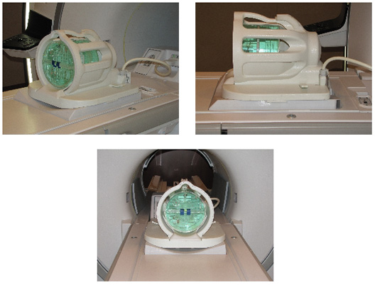
Figure 7. Example of Positioning of Phantom in Head Coil 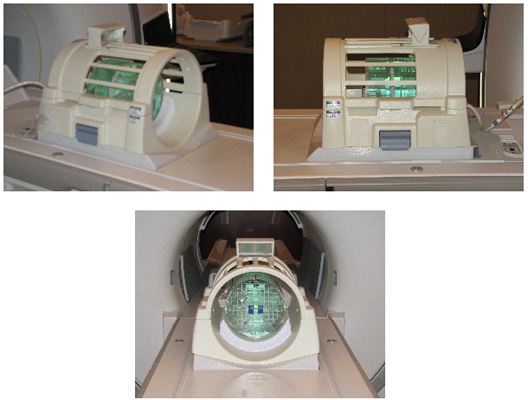
-
ACR Sagittal Localizer Series
-
Select Add Task, then Add Sequence.
-
For an HDx system: proceed to Step 6.
For a DV system: To access the Protocol Library, click GE
-
On the Template tab, open the 2D Spin Echo folder, select Spin Echo series, and then click the right arrow button.
-
Under Multi Protocol Basket, select Spin Echo series, and then click Accept.
-
On the Task tab, select Spin Echo series, and then click Setup.
-
Select the Spin Echo series and rename it ACR Sagittal Localizer.
-
Prescribe the ACR Sagittal Localizer series as follows:
Coil {selected head-type coil} Orientation Head First, Supine Imaging Options Plane: Sagittal
Mode: 2D
Family: Spin Echo
Pulse: Spin Echo
Application: None
Imaging Option: None
PSD Name: leave blank
Scan Plane Sagittal Freq. FOV 25.0 Phase FOV 1.00 Slice Thickness 20.0 Spacing 0.0 Freq. Dir S/I TR 200 # Slices 1 Start R/L: If the phantom was earlier centered to within ±1mm along L/R, then enter 0 for both the Start and End R/L offsets. If the phantom could not be centered ±1mm, then enter the previously determined offset for both the Start and End R/L offsets. Use either R or L (specifies direction), immediately preceding the number of millimeters to offset.
P/A: 0.0
I/S: 0.0
End R/L: If the phantom was earlier centered to within ±1mm along L/R, then enter 0 for both the Start and End R/L offsets. If the phantom could not be centered ±1mm, then enter the previously determined offset for both the Start and End R/L offsets. Use either R or L (specifies direction), immediately preceding the number of millimeters to offset.
P/A: 0.0
I/S: 0.0
Chem SAT None Contrast Off (deselect) # of TE(s) per Scan 1 TE 20.0 Intensity Correction NONE for TR Head Coil, otherwise SCIC Intensity Filter NONE 3D Geom. Correction Default (deselected) Frequency 256 Phase 256 NEX 1.00 Bandwidth 15.63 Shim Auto RF Drive Mode (if present) Default Phase Correct Default (off) Table delta Default (0.0) -
Auto Prescan and Scan.
-
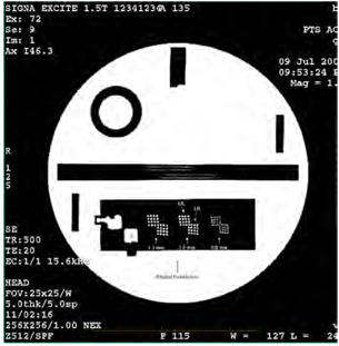
View the resulting ACR sagittal localizer image and verify that the phantom appears as below.
Figure 8. Example for ACR Sagittal Localizer Series 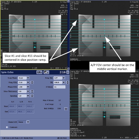
ACR T1 series
-
Copy and paste the previous ACR Sagittal Localizer series and rename the new one ACR T1.
-
Prescribe the ACR T1 series as follows:
Coil {selected head-type coil} Orientation Head First, Supine Imaging Options Plane: Axial
Mode: 2D
Family: Spin Echo
Pulse: Spin Echo
Application: None
Imaging Option: None
PSD Name: leave blank
Scan Plane Axial Freq. FOV 25.0 Phase FOV 1.00 Slice Thickness 5.0 Spacing 5.0 Freq. Dir A/P TR 500 # Slices 11 (1 > 11, Inferior to Superior) Start S/I: (graphic Rx will fill in automatically)
L/R: (graphic Rx will fill in automatically)
P/A: (graphic Rx will fill in automatically)
End S/I: (graphic Rx will fill in automatically)
L/R: (graphic Rx will fill in automatically)
P/A: (graphic Rx will fill in automatically)
Graphic Rx -
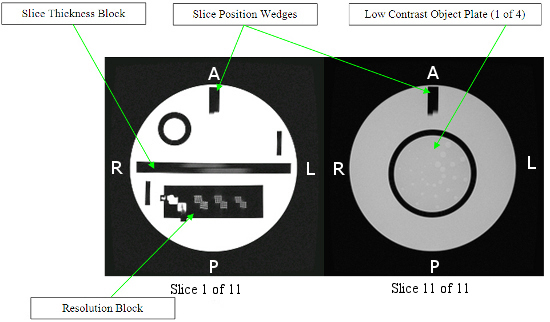
Using the ACR sagittal localizer from above, place the starting axial slice (1) through the vertex of the crossed wedge at the CHIN (inferior) end of the phantom and the last slice (11) through the vertex of the crossed wedge at the NOSE (superior) end of the phantom.
-
Adjust the graphic Rx to balance the first and last of the 11 axial slices on these two vertices.
-
The planes of slices 8, 9 10, and 11 should approximately align on the 4 low contrast discs at the Superior end of the phantom.
Chem SAT None Contrast Off (deselect) # of TE(s) per Scan 1 TE 20.0 Intensity Correction NONE for TR Head Coil, otherwise SCIC Intensity Filter NONE 3D Geom. Correction Default (deselected) Frequency 256 Phase 256 NEX 1.00 Bandwidth 15.63 Shim Auto RF Drive Mode (if present) Default Phase Correct Default (off) Table delta Default (0.0) -
-
Auto Prescan and Scan.
-
View the resulting first image of the ACR T1 series and verify that the phantom appears as below.
Figure 9. Example of ACR T1 Series 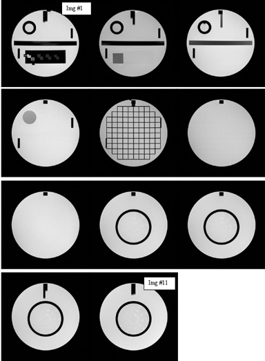
ACR T2 series
-
Copy and paste the previous ACR T1 series and rename the new one ACR T2.
-
Prescribe the ACR T2 series as follows:
Coil {selected head-type coil} Orientation Head First, Supine Imaging Options Plane: Axial
Mode: 2D
Family: Spin Echo
Pulse: Spin Echo
Application: None
Imaging Option: None
PSD Name: leave blank
Scan Plane Axial Freq. FOV 25.0 Phase FOV 1.00 Slice Thickness 5.0 Spacing 5.0 Freq. Dir A/P TR 2000 # Slices 11 (1 > 11, Inferior to Superior) Center S/I: (graphic Rx will fill in automatically)
L/R: (graphic Rx will fill in automatically)
P/A: (graphic Rx will fill in automatically)
Spacing S/I: (graphic Rx will fill in automatically)
L/R: (graphic Rx will fill in automatically)
P/A: (graphic Rx will fill in automatically)
Graphic Rx: Use the localizer and stored Graphic Rx used for the ACR T1 series above (exact same slice locations, FOV). Chem SAT None Contrast Off (deselect) # of TE(s) per Scan 2 TE 20.0 TE2 80.0 Intensity Correction NONE for TR Head Coil, otherwise SCIC Intensity Filter NONE 3D Geom. Correction Default (deselected) Frequency 256 Phase 256 NEX 1.00 Bandwidth 15.63 Bandwidth2 15.63 Shim Auto RF Drive Mode (if present) Default Phase Correct Default (off) Table delta Default (0.0) -
Auto Prescan and scan.
-
View the resulting first image and verify that the phantom object is correct. The ACR T2 images should look the same as the ACR T1 images, except there are two images/echoes per slice. (See Figure 9.)
Saving results
Save the 3-plane localizer series, ACR sagittal localizer series, ACR T1 series, and ACR T2 series images to media and label them with the site/system name, operator name, date, exam/series/images, field strength, software version, and ACR phantom number(s).
ACR Phantom Image Analysis
ACR phantom analysis is done by manual measurements on the resulting images and can be somewhat subjective. It is important to follow the ACR guidelines closely and work carefully when doing the measurements to get the most accurate measurements possible.
Following are summaries of the ACR phantom measurement procedures using GE Signa generated example images. For detailed explanations of each ACR phantom measurement, refer to the Phantom Test Guidance document published by the ACR and available on the ACR website (www.acr.org).
There are seven ACR phantom image measurements required. Some of the measurements are required on multiple images. The seven measurements are as follows:
-
Geometric accuracy
-
High contrast spatial resolution
-
Slice thickness accuracy
-
Slice position accuracy
-
Image intensity uniformity
-
Percent signal ghosting
-
Low contrast object detectability
Geometric Accuracy
Geometric accuracy checks the accuracy of the gradient gain calibration (Grad Cal adjustment).
Sagittal Localizer – S/I Distance Measurement
-
Display the ACR sagittal localizer image.
-
Adjust the window width (WW) to the most narrow setting (0).
-
Slowly lower the Window Level just enough until the signal in the “water-only” region (that with brightest relative signal, not partial-volumed by internal phantom structures) is all white.
-
Raise the Window Level until about half of the water-only region has turned black.
The resulting ACR Sagittal Localizer Reference Window Level approximates the mean signal value in the water-only regions.
-
Record the ACR Sagittal Localizer Reference Window Level on the ACR Accreditation Scan Measurements form provided in ACR Phantom Scanning.
-
Set the display Window Level to one half the ACR Sagittal Localizer Reference Window Level.
-
Set the Window Width to the ACR Sagittal Localizer Reference Window Level.
-
Using the ACR Sagittal Localizer, measure in mm the end-to-end length (along the S/I direction) of the ACR phantom along a line which lies on the 5th of 11 small dark segments (numbered from left to right on the image’s A/P axis).
Note:WW is not adjusted correctly in the example image below, so that line plot location is easier to see.
Figure 10. Sagittal Localizer S/I Distance Measurement 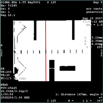
-
Record this as ACR Sagittal Localizer S/I Length in the ACR Accreditation Scan Measurements form.
-
Verify that ACR Sagittal Localizer S/I Length is 148 mm ± 2 mm.
Axial T1 Slice 1 A/P and R/L Distance Measurements
-
Display the ACR T1 series images in the viewer.
-
On ACR T1 series slice 1 (the most inferior axial location), measure the phantom's diameter in the R/L direction (horizontal in image) on top of the grid's horizontal center line.
Note:WW is not adjusted correctly in the example image below, so that line plot location is easier to see.
Figure 11. Axial T1 A/P and R/L Distance Measurements 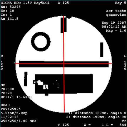
-
Record this ACR T1 End Slice R/L Diameter in the ACR Accreditation Scan Measurements form provided in ACR Phantom Scanning.
-
On ACR T1 series slice 1 (the most inferior axial location), measure the phantom's diameter in the A/P direction (vertical in image) on top of the grid's vertical center line.
Notice -
Record this ACR T1 End Slice A/P Diameter in the ACR Accreditation Scan Measurements form.
-
Verify that both distance measurements are equal to 190 mm ±2 mm.
Axial T1 Slice 5 A/P, R/L, +45, and –45 Distance Measurements
-
On ACR T1 Series slice 5 (the center axial location), measure the phantom's diameter along the four (4) directions: R/L, A/P, +45 degree diagonal (positive slope) and -45 degree diagonal (negative slope).
Note:WW is not adjusted correctly in the image below, so that line plot location is easier to see.
Figure 12. A/P, R/L, +45, and -45 Diameter of Phantom Image 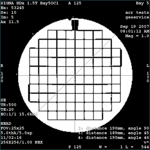
-
Record these values in the ACR Accreditation Scan Measurements form.
-
Verify that all four distance measurements are equal to 190 mm ±2 mm.
High Contrast Spatial Resolution (8HRBrain Coil)
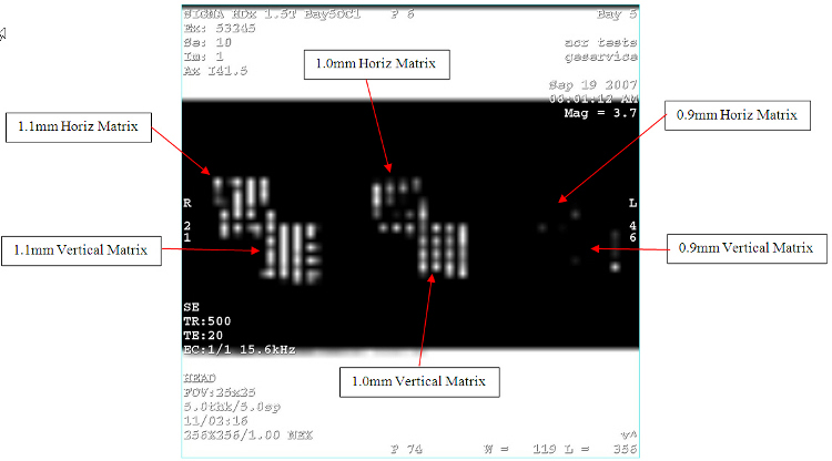
The ACR T1 series image slice 1, shown in the illustration below, contains a horizontally oblong dark resolution block in the lower half of the phantom.
Note that when you’re looking at the Upper Left matrix of dots in each pair of matrices, and trying to assess whether 4 things can be distinctly seen going across (left/right) in a particular row, it doesn’t matter if any or all of the dots in that particular row are blurred into, bridged to, or combined with a dot from an adjacent row above or below the row being examined As long as you can distinguish 4 distinct bright objects in the row being examined, it passes in the’ Left/Right direction for that particular resolution value. Note that only 1 row (at least one row) of the 4 rows in the Upper Left matrix needs to be visualized as just described in order for that resolution to pass”.
When looking at the Lower Right matrix of dots in each pair of matrices the process is analogous to that described above but instead of examining 4 rows you are examining 4 COLUMNS and looking for resolution in the Top-bottom direction. You can also refer to ACR’s Large Phantom Guidance documents at acr.org for additional details.
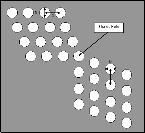
Each UL array in a pair comprises 4 rows of 4 holes each. The center-to-center hole separation within each row AND the center-to-center row separation are both twice the hole diameter. Each row is staggered slightly to the right of the one above, which is why the array is not quite square.
Each LR array in a pair comprises 4 columns of 4 holes each. The center-to-center hole separation within each column and the center-to-center spacing between each columns are both twice the hole diameter. Each column is staggered slightly downward from the one to its left.The hole diameter differs between the 3 pairs of arrays. The left pair has 1.1 mm holes, the center pair has 1.0 mm holes and the right pair has 0.9 mm holes.
-
Display the ACR T1 series images.
-
On ACR T1 series slice 1 (the most inferior slice location), magnify the image by a factor of 2 to 4.
-
Viewing the UL array of the 1st array pair (left most pair of 3 pair) with the 1.1 mm hole diameter, adjust the Window Width and Window Level to best resolve the 4 holes in any single row (R/L direction) of this UL array.
-
If all 4 holes in any of its single rows are distinguishable from one another, then record ACR T1 Left-Right resolved @1.1 mm as “Yes.” If not, record it as “No.” Use the ACR Accreditation Scan Measurements form provided in ACR Phantom Scanning.
-
Viewing the LR array of the 1st array pair (left most pair of 3 pair) with the 1.1 mm hole diameter, adjust the Window Width and Window Level to best resolve the 4 holes in any single column (top-bottom or A/P direction) of this LR array.
-
If all 4 holes in any of its single columns are distinguishable from one another, then record ACR T1 Top-Bottom resolved @1.1 mm as “Yes.” If not, record it as “No.” Use the ACR Accreditation Scan Measurements form to record the values.
-
Repeat steps 3 & 4 but for the 2nd array pair (middle pair of 3 pair) and record the status of ACR T1 Left- Right resolved @1.0mm and ACR T1 Top-Bottom resolved @1.0 mm. Use the ACR Accreditation Scan Measurements form to record the values.
-
Repeat steps 3 & 4 but for the 3rd array pair (last pair of 3 pair) and record the status of ACR T1 Left- Right resolved @0.9mm and ACR T1 Top-Bottom resolved @0.9 mm . Use the ACR Accreditation Scan Measurements form to record the values.
-
Repeat steps 1-6 but use the ACR T2 series slice 1 image, 2nd echo only. Record the analogous results. Use the ACR Accreditation Scan Measurements form to record the values.
Note:The “resolved@0.9mm” observed outcomes for T2 do not have to be checked “Yes” for the test to pass.
-
If the ACR T1 and ACR T2 images analyzed are resolved in both the Left-Right and Top- Bottom directions to at least 1.0mm (i.e. resolved at both 1.1mm and 1.0mm), the High Contrast Spatial Resolution Test has passed.
Slice Thickness Accuracy (8HRBrain Coil)
The ACR MRI phantom contains a horizontally oblong structure (in the center CORONAL plane) called the slice thickness insert within which there are 2 horizontally oriented signal ramps. The length of these 2 ramps will be measured and used to calculate the slice thickness in mm.
-
Display the ACR T1 series images.
-
On the ACR T1 series slice 1 (the most inferior location), magnify the image by a factor of 2 to 4, keeping the phantom's slice thickness insert and its 2 signal ramps fully visible.
The ramp signal level is much lower than that of the water surrounding the slice thickness insert, so it will be necessary to lower the Window Level and Window Width to well visualize both signal ramps.
-
Place a rectangular ROI of approximate width 21mm (~22 pixels), with its center at the approximate horizontal center of the top signal ramp.
Make sure the vertical size of this ROI covers the width of the top ramp in the top-bottom direction but does not include low signal pixels above or below the TOP ramp itself.
-
Record the ROI mean signal value as ACR T1 Top Ramp ROI mean in the ACR Accreditation Scan Measurements form provided in ACR Phantom Scanning.
-
Repeat this ROI measurement as detailed above using the same ROI horizontal width but for the bottom signal ramp and record the ROI mean signal value as ACR T1 Bottom Ramp ROI mean. Use the ACR Accreditation Scan Measurements form to record the values.
-
Set the Window Level to one half the average of the previously calculated ROI means and set the Window Width to minimum.
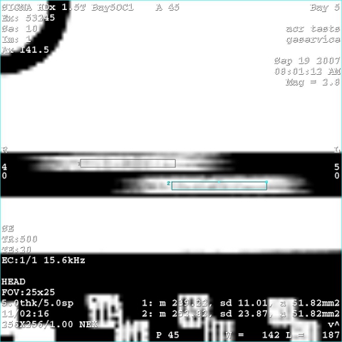
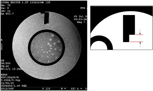
At this display setting, there are often horizontal striations in a ramp’s signal that cause its ends to appear scalloped or ragged. In this case one must estimate the average locations of the ramp’s ends in order to measure its length. See the illustration below as an example of how the measurement should be made under this condition.
Figure 17. Slice Thick Ramp Distance Measurements 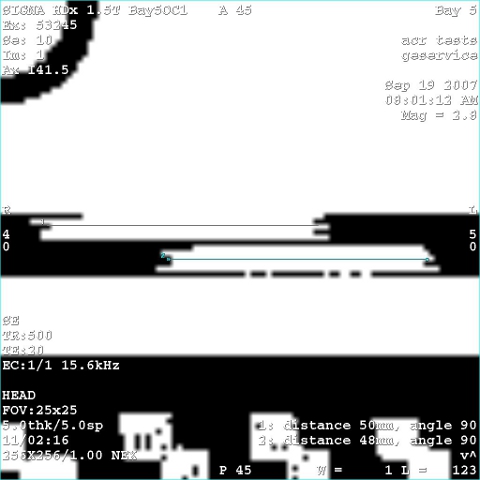
-
Use the on-screen measurement tool to measure and record the top ramp’s length in mm as ACR T1 Top Ramp Length to the right. Repeat the measurement for the bottom ramp and record as ACR T1 Bottom Ramp Length. Use the ACR Accreditation Scan Measurements form to record the values.
-
Calculate the slice thickness using the following formula:
slice thickness = 0.2 x (top x bottom) / (top + bottom)
where top and bottom refer to the ACR T1 Top Ramp Length (mm) and ACR T1 Bottom Ramp Length (mm) respectively.
-
Record the calculated value as ACR T1 Slice Thickness (mm). Use the ACR Accreditation Scan Measurements form to record the values.
-
Repeat these steps using the ACR T2 series slice 1 (most inferior location) using the 2nd echo image. Record the analogous values. Use the ACR Accreditation Scan Measurements form to record the values.
-
If both the ACR T1 & T2 series slice thicknesses are equal to 5.0mm ±0.7mm, the Slice Thickness Accuracy Test has passed.
Slice Position Accuracy
The slice position accuracy test assesses the accuracy with which slices can be prescribed at specific locations utilizing the localizer image for positional reference.
Slices 1 and 11 were prescribed to be aligned with the vertices of the crossed 45 degree wedges at the inferior and superior ends of the phantom respectively. On the images of slices 1 and 11 the crossed wedges appear as a pair of adjacent, dark vertical bars at the top (anterior side) of the phantom. See illustration below. A perfectly positioned slice’s image shows a dark bar pair with left and right sides of equal vertical length. If the slice is displaced superiorly with respect to the vertex, the bar on the observer’s right (anatomical left) is longer. If the slice is displaced inferiorly with respect to the vertex, the bar on the left (anatomical right) will be longer.
-
Display the ACR T1 series images.
-
On ACR T1 series slice 1 (most inferior location), magnify the image by a factor of 2 to 4, keeping the vertical bars of the crossed wedges within the displayed portion of the magnified image.
-
Adjust Window Width to 1 (the most narrow setting).
-
Slowly lower the Window Level just enough until the signal in the “water-only” region (that with brightest relative signal, not partial-volumed by internal phantom structures) is all “white.”
-
Now raise the Window Level until about half of the water-only region has turned “black.”
-
Use the measure distance function to measure the lengths of the left and right slice position wedges.
This resulting ACR T1 Slice 1 Ref Window Level approximates the mean signal value in the water-only regions.
-
Record the ACR T1 Slice 1 Ref Window Level in the ACR Accreditation Scan Measurements form provided in ACR Phantom Scanning.
-
Set the Window Level to one half of the ACR T1 Slice 1 Ref Window Level. Adjust the Window Width to a low value so the ends of the vertical bars are well defined (not fuzzy).
-
Referring to Figure 18, use the on-screen length measurement tool to measure the difference in vertical lengths between the left & right bars of the cross wedge in mm.
-
Record the difference (as a negative value if the left bar is longer) as ACR T1 Slice 1 Bar Length Difference (mm). Use the ACR Accreditation Scan Measurements form to record the values.
-
Repeat steps 1-9 for ACR T1 series slice 11 and record the analogous values. Use the ACR Accreditation Scan Measurements form to record the values.
-
Repeat steps 1-10 using the ACR T2 series slices 1 & 11, 2nd echo only. Record the ACR T2 series analogous values. Use the ACR Accreditation Scan Measurements form to record the values.
-
If the absolute value of the ACR T1 slice 1 & 11 and ACR T2 slice 1 & 11 bar length differences (4 of them) are all 5.0 mm, the Slice Position Accuracy Test has passed.
Image Intensity Uniformity
The image intensity uniformity test measures the uniformity of the image intensity over a large water-only region of the phantom lying near the middle of the imaged volume and thus near the middle of the head coil.
-
Display the ACR T1 series image for slice 7.
-
Center a circular ROI (approximately on the phantom but not including the top black rectangle) with an area between 195cm2 and 205cm2 (19,500 mm2 to 20,500 mm2) as shown in the following illustration.
It is recommended that you get as close as possible to 20000 mm^2” to be in the middle of the size range. Make sure the ROIs top edge is at least three pixels below the black rectangle’s bottom edge.
Figure 19. Intensity Uniformity Low Signal ROI Placement 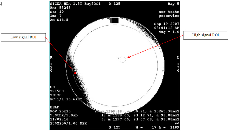
-
Set the Window Width to minimum and lower the Window Level until the entire ROI area is “white.”
-
Now raise the Window Level until a small 100 mm2 region of dark pixels develops inside the ROI.
If more than one dark region develops, focus on the largest one. If you end up with 1 or more wide, poorly defined dark areas or areas of mixed black and white pixels, then make a visual estimate of the location of the darkest 100mm2 portion of the largest dark area.
-
Place a small circular ROI (roughly 100 mm2) on this dark region as in Figure 10 at the beginning of the ACR section.
If there is uncertainty about where to place the ROI because there is no single obviously darkest location, try several locations and select the one having the lowest pixel mean.
-
Record this ROI signal mean as ACR T1 ROI_Low Signal Mean in the ACR Accreditation Scan Measurements form provided in ACR Phantom Scanning.
-
Now continue to raise the Window Level until only a small roughly 100mm2 area region of white pixels remains inside the large base ROI.
If more than one bright region remains, focus on the largest one. If you end up with 1 or more diffuse areas of mixed black and white pixels, then make a visual estimate of the location of the brightest 100 mm2 area portion of the largest bright area.
-
Place a 2nd small circular ROI (roughly 100 mm2 area) on this white region as in Figure 11 at the beginning of the ACR section.
If there is uncertainty about where to place the ROI because there is no single obviously brightest location, try several locations and select the one having the highest pixel mean.
-
Record this ROI signal mean value as ACR T1 ROI_High signal mean. Use the ACR Accreditation Scan Measurements form to record the values.
-
Calculate the Percent Integral Uniformity (PIU) with the following formula:
PIU = 100 x [1 – {(high – low) / (high + low)}]
where high and low represent the ACR T1 ROI-High signal mean and ACR T1 ROI-Low signal mean respectively.
-
Record the calculated PIU value as ACR T1 PIU (%). Use the ACR Accreditation Scan Measurements form to record the values.
-
Repeat steps 1-5 using the ACR T2 image series slice 7, 2nd echo only. Record the ACR T2 series analogous values. Use the ACR Accreditation Scan Measurements form to record the values.
-
Verify the ACR T1 and T2 PIU values.
For 1.5T systems, verify that the ACR T1 and T2 PIU >= 87.5%.
For 3.0T systems, verify that the ACR T1 and T2 PIU >= 82.0%.
If the percentages are correct, the Image Intensity Uniformity Test has passed.
Percent Signal Ghosting
The Percent-Signal Ghosting test assesses the level of ghosting in the images. Ghosting is an artifact in which a faint copy (ghost) of the imaged object appears superimposed on the image, displaced from its true location. If there are many low level ghosts, they may not be recognizable as copies of the object but simply appear as a smear of signal emanating in the phase encode direction from the brighter regions of the true image. For this test, the ghost signal level is measured and reported as a percentage of the signal level in the true (primary) image.
-
Display the ACR T1 series image of slice 7.
-
Center a circular ROI (approximately on the phantom but not including the top black rectangle) with an area between 195 cm2 and 205 cm2 (19,500 mm2 to 20,500 mm2) as in the illustration below.
Figure 20. Ghost Measurement ROI Placements 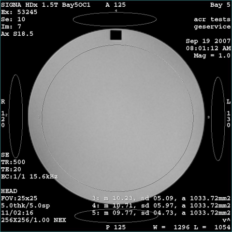
-
Record the ROI s mean as ACR T1 ROI_Large Signal Mean in the ACR Accreditation Scan Measurements form provided in ACR Phantom Scanning.
-
Place four elliptical background ROI s, each with about a 4:1 length-to-width (i.e. long-to-short) aspect ratio and area of about 1000 mm2, each centered between but not touching their adjacent field-of-view and phantom edges. See Figure 20.
It is important to prevent the ROIs from touching a phantom edge or from including any true zero background border (caused by recon’s gradwarp process) that may be at the FOV edge. If the phantom is off center in the FOV, it may be necessary to reduce the width of some of the ROIs to fit them between the phantom and the edge of the FOV. If this is so, reduce the ROI width as necessary to fit and increase its length to maintain an approximate 1000 mm2 area.
-
Record the ROI mean values as ACR T1 ROI_[top, bottom, left, right] Signal Mean. Use the ACR Accreditation Scan Measurements form to record the values.
-
Calculate the ghosting ratio using the following formula:
ghosting ratio = | ( (top + bottom) - (left + right) ) / ( 2 x (ROI_Large) ) |
Note:Vertical bars (|) indicate magnitude of enclosed value.
-
Record the ghosting ratio value as ACR T1 Ghosting Ratio. Use the ACR Accreditation Scan Measurements form to record the values.
-
Verify that the ghosting ratio <= 0.025.
Low Contrast Object Detectability
The low-contrast object detectability test assesses the extent to which objects of low contrast are discernible in the images. For this purpose, the phantom has a set of low contrast objects of varying size and contrast.
The low contrast objects appear on slices 8, 9, 10 & 11 with contrast ratios of 1.4%, 2.5%, 3.6%, and 5.1% respectively per slice. In each slice, the low contrast objects appear as rows of small disks radiating from a center hub like spokes on a wheel. Each wheel (one per slice) is composed of 10 spokes and each spoke is composed of 3 same sized disks along its length. The largest disks are 7.0 mm in diameter on spoke 1 at its approximate one o’clock position. The disk size progressively decreases to a minimum of 1.5 mm on last spoke 10 at its approximate 11:30 position as the spokes progress clockwise.
-
Display the ACR T1 series slice 11 image.
-
Adjust Window Level to visualize the low contrast objects, keeping the Window Width fairly narrow.
Figure 21. Low Contrast Object Spokes 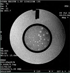
-
Starting at spoke 1 at the one o’clock position, count clockwise until a spoke is reached where one or more disks on it are not discernible from the background.
-
Record the number of complete spokes that can be visualized, up to but not including the indiscernible spoke, as ACR T1 Slice 11 Complete Spokes. Use the ACR Accreditation Scan Measurements form provided in ACR Phantom Scanning.
-
Repeat steps 1-3 for ACR T1 series slices 10, 9 & 8.
-
Record the slice 10, 9 & 8 analogous values. Use the ACR Accreditation Scan Measurements form to record the values.
-
Total up the spokes for all 4 slices analyzed from the ACR T1 series and record it as ACR T1 Total Spokes. Use the ACR Accreditation Scan Measurements form to record the values.
-
Repeat steps 1-5 using the ACR T2 image series slices 11, 10, 9 & 8, each 2nd echo only. Record the analogous ACR T2 series values. Use the ACR Accreditation Scan Measurements form to record the values.
-
Verify that Low Contrast Object Detection passes.
For 1.5T systems, 9 spokes must be visible.
For 3.0T systems, 37 spokes must be visible.
Tips for 1.5T and 3.0T Cylindrical Scanners
Phantom Positioning
With a properly calibrated system and properly positioned ACR phantom, 1.5T and 3.0T systems should not have any problems passing the ACR phantom measurement tests. Many reported failures from 1.5T and 3.0T systems have been primarily due to ACR phantom positioning. It is critical that the prescribed slices in the ACR T1 and T2 protocols match the phantom structures as close as possible, and therefore proper phantom positioning is critical. Use the iterative 3-plane localizer technique outlined above to achieve proper phantom positioning.
Patient Weight and Effect on Number of Acquisitions
The patient weight parameter is set at 50 pounds to ensure a single acquisition pass. Higher weights would break the scan into two acquisitions, which increases scan time. Because acquisition time is one of several parameters that is considered in the ACR evaluation, it is important to keep the weight low to maintain a single acquisition pass.
Failures on TWIN Gradient Coil Systems
On systems with a TWIN gradient coil (WHOLE and ZOOM mode), use one gradient mode exclusively when performing ACR phantom testing. Do not switch between WHOLE and ZOOM modes. Normally, the ZOOM gradient mode is used for head coil scanning. There are slight spatial accuracy differences between the WHOLE and ZOOM gradient modes because of different slew rates, gradient linearities, and grad warp corrections.
Graphic Rx
The ACR phantom scanning instructions specify using Graphic Rx when prescribing the 11 slices on the ACR sagittal localizer image. The pixel dimension in the sagittal localizer is 0.976 mm2. The Graphic Rx screen uses slightly less than a quarter of the screen to display the sagittal localizer image when graphically prescribing the slices. Very small movements of 1 pixel on the graphic Rx lines correlate to almost a millimeter of slice location placement. Small slice location errors can be induced if the Graphic Rx lines are not placed perfectly over the sagittal localizer. Using the manual slice location prescription method described in Slice Position Accuracy sometimes provides better slice position accuracy.
Autoshim and Effects on Image Uniformity and Low Contrast Object Detection
In at least one instance on a 3.0T scanner, turning off Autoshim produced better image intensity uniformity and better low contrast object detection results. In this case, LVshim Grad Shim was run first to optimize the grad shim compensation, then the test was run with and without Autoshim enabled. Autoshim appeared to be making large adjustments to the default grad shim values and causing more intensity variations in the resulting images. Turning off Autoshim and using the default optimized grad shim numbers produced more uniform images, making the image intensity uniformity and low contrast object detection measurements better.
Using SCIC or PURE for 3.0T Image Uniformity
3.0T systems have more difficulty with image intensity uniformity because of standing wave effects and the electrical properties of the ACR phantom. It is completely acceptable to the ACR to use SCIC or PURE filtering to improve image intensity uniformity at 3.0T.
Alignment Lights and Table Movements Causing Positioning Errors
In a few instances, axial alignment lights have been observed that were not perfectly vertical and projected downward at some angle. This angle induces an isocenter calibration error dependent on the height of the phantom used. Then after prescribing the axial slices, the table is required to move in the S/I direction. If there is mechanical slop in the table or table encoder problems, the table does not move to the correct location with enough accuracy. This causes slice position errors in the ACR phantom scans and subsequent test failures. To avoid this, verify that the axial alignment lights are properly adjusted, table movements are in specification, and isocenter calibration is in specification and is repeatable.
Artifacts
Any noticeable artifacts (ghosting, zippers, correlated noise, etc.) in any of the ACR images may cause the ACR reviewer to fail the images. There are no specific measurements for artifacts other than the ghosting measurements, but even if all ACR phantom tests pass, the presence of any artifacts can still cause the ACR reviewer to fail the images.
2–3 mm Differences on Bar Length Measurements
If the bar length difference for slice 1 and slice 11 are the same in sign and similar in magnitude, the cause may be the position of the table.
Try the following to close the difference.
-
Adjust the belt tension.
-
Check that the laser alignment is vertical.
-
Confirm that the table is latched to the carriage.
-
Check the isocenter calibrations.
Images are now almost too close to measure. For image 11, the difference is likely less than 1 mm; for image 1, 0 mm. The test is VERY sensitive to correct positioning of the phantom.
For detail information about correct positioning to get a good Slice Position Accuracy Test, see Slice Position Accuracy
Low Contrast Object Detection (LCOD)
Possible solutions for Low Contrast Object Detection (LCOD) are
-
Axial slice GRx S/I positioning (slices too superior, not close enough to LCOD disks).
When graphically prescribing (positioning) the ACR T1 protocol’s 11 axial slices on the sagittal ACR Localizer, you may need to place the 11th slice slightly lower (slightly inferior to) the upper vertex so any GAP between slices 11, 10 , 9 and 8 and their respective Low Contrast Object Detection discs is narrower. This may amount to offsetting the 11th slice about 1 or 2 of the smallest possible GRx positioning “steps” downward from its ideal location at the center of the vertex, but just enough to narrow the aforementioned GAP without compromising the Slice Position Accuracy test results to the point of failure. The closer slices 11, 10, 9 and 8 are to their respective LCOD discs, the better the visibility of spokes in the LCOD test.
-
Incrementing TG may help improve results.
-
Phantom positioning (object rotated slightly clockwise in Sagittal, slightly clockwise in Axial).
Increased TG and Effects on Image Uniformity
(For 3T scanning only) Due to the dielectric shading and loading effects with the ACR phantom in the 3T TR Head coil, the Percent Image Uniformity or “PIU” tests (for ACR T1 series slice 7 and/or ACR T2 series slice 7, echo 2) may not pass with the default Auto PreScan TG values. If it does not pass, try incrementing the APS TG value in multiples of 4 (for example, first by 4, then 8, etc.) to reduce shading and pass PIU.
Bubbles in Phantom and Effect on Measurements
If the ACR phantom contains a bubble, be careful when making any measurements to ensure that the bubble is not affecting those measurements. For instance, when taking geometric accuracy measurements (see Geometric Accuracy), a bubble at the very top of the axial image could prevent you from making an accurate A/P length measurement.
| Notice | |
|---|---|